


Databricks Related Exams
Last Week Results
32 Customers Passed Databricks
Databricks-Certified-Professional-Data-Scientist Exam
Databricks-Certified-Professional-Data-Scientist Exam
Average Score In Real Exam
Questions came word for word from this dump

Databricks Bundle Exams
Duration: 3 to 12 Months
4 Certifications
12 Exams
Databricks Updated Exams
Most authenticate information
Prepare within Days
Time-Saving Study Content
90 to 365 days Free Update
$249.6*

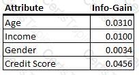
 Table
Description automatically generated
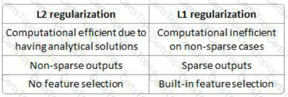
Table
Description automatically generated